[Sorry for the delay in this post. I was having some difficulties coming up with some of the rationales below. Also, classes have started, which has made me very busy.]
If there was one ODE solving method that I did not want to implement this summer, it was undetermined coefficients. I didn’t really like the method too much when we did it my my ODE class (though it was not as unenjoyable as series methods). The thing that I never really understood very well is to what extent you have to multiply terms in the trial function by powers of x to make them linearly independent of the solution to the general equation. We did our ODEs homework in Maple, so I would usually just keep trying higher powers of x until I got a solution. But to implement it in SymPy, I had to have a much better understanding of the exact rules for it.
From a user’s point of view, the method of undetermined coefficients is much better than the method of variation of parameters. While it is true that variation of parameters is a general method and undetermined coefficients only works on a special class of functions, undetermined coefficients requires no integration or advanced simplification, so it is fast (very fast, as well shall see below). All that the CAS has to do is figure out what a trial function looks like, plug it into the ODE, and solve for the coefficients, which is a system of linear equations.
On the other hand, from the programmer’s point of view, variation of parameters is much better. All you have to do is take the Wronskian of the general solution set and use it to set up some integrals. But the Wronskian has to be simplified, and if the general solution contains sin’s and cos’s, this requires trigonometric simplification not currently available in SymPy (although it looks like the new Polys module will be making a big leap forward in this area). Also, integration is slow, and in SymPy, it often fails (hangs forever).
Figuring out what the trial function should be for undetermined coefficients is way more difficult to program, but having finnally finished it, I can say that it is definitely worth having in the module. Problems that it can solve can run orders of magnitude faster than the variation of parameters, and often variation of parameters can’t do the integral or returns a less simplified result.
So what is this undetermined coefficients? Well, the idea is this: if you knew what each linearly independent term of the particular solution was, minus the coefficients, then you could just set each coefficient as an unknown, plug it into the ODE, and solve for them. It turns out that resulting system of equations is linear, so if you do the first part right, you can always get a solution.
The key thing here is that you know what form the particular solution will take. However, you don’t really know this ahead of time. All you have is the linear ode 


It turns out that this method only works if the function 


So this gives us the exact form of functions that we need to look for to apply undetermined coefficients, based on the assumption that it only works on functions with a finite number of linearly independent derivatives.
Well, implementing it was quite difficult. For every ODE, the first step in implementation is matching the ODE, so the solver can know what methods it can apply to a given ODE. To match in this case, I had to write a function that determined if the function matched the form given above, which was not too difficult, though not as trivial as just grabbing the right hand side in variation of parameters. The next step is to use the matching to format the ODE for the solver. In this case, it means finding all of the finite linearly independent derivatives of the ODE, so that the solver can just create a linear combination of them solve for the coefficients. This was a little more difficult, and it took some lateral thinking.
At this point, there is one more thing that needs to be noted. Since the trial functions, that is, the linearly independent derivative terms of the right hand side of the ODE, are of the same form as the solutions to the homogeneous equation, it is possible that one of the trial function terms will be a solution to the homogeneous equation. If this happens, plugging it into the ODE will cause it to go to zero, which means that we will not be able to solve for a coefficient for that term. Indeed, that term will be of the form 
We can safely ignore these terms for undetermined coefficients, because their coefficients will not even appear in the system of linear equations of the coefficients anyway. But, without these coefficients, we will run into trouble. It turns out that if a term 


Most references simply say that you need to multiply the trial function terms by “sufficient powers of x” to make them linearly independent with the homogeneous solution. Well, this is just fine if you are doing it by hand or you are creating the trial function manually in Maple and plugging it in and solving for the coefficients. You can just keep upping the powers of x until you get a solution for the coefficients. Creating those trial functions in Maple, plugging them into the ODE, and solving for the coefficients is exactly what I had to do for my homework when I took ODEs last spring, and this “upping powers” trial and error method is exactly the method I used. But when you are doing it in SymPy, you need to know exactly what power to multiply it by. If it is too low, you will not get solution to the coefficients. If it is too high, you can actually end up with too many terms in the final solution, giving a wrong answer.
Fortunately, my excellent ODEs textbook gives the exact cases to follow, and so I was able to implement it correctly. The textbook also gives a whole slew of exercises, all for which the solutions are given. As usual, this helped me to find the bugs in my very complex and difficult to write routine. It also helped me to find a match bug that would have prevented dsolve() from being able to match certain types of ODEs. The bug turned out to be fundamental to the way match() is written, so I had to write my own custom matching function for linear ODEs.
The final step in solving the undetermined coefficients is of course just creating a linear combination of the trial function terms, plugging it into the original ODE, and setting the coefficients of each term on each side equal to each other, which gives a linear system. SymPy can solve these easily, and once you have the values of the coefficients, you can use them to build your particular solution, at which point, you are done.
The results were astounding. Variation of parameters would hang on many simple inhomogeneous ODEs because of poor trig simplification of the Wronsikan, but my undetermined coefficients method handles them perfectly. Also, there is no need to worry about absorbing superfluous terms into the arbitrary constants as with variation of parameters, because they are removed from within the undetermined coefficients algorithm.
But the biggest thing was speed. Here are some benchmarks on some random ODEs from the test suite. WordPress code blocks are impervious to whitespace, as I have mentioned before, so no pretty printing here. Also, it truncates the hints. The hints used are 'nth_linear_constant_coeff_undetermined_coefficients' and 'nth_linear_constant_coeff_variation_of_parameters':
In [1]: time dsolve(f(x).diff(x, 2) - 3*f(x).diff(x) - 2*exp(2*x)*sin(x), f(x), hint='nth_linear_constant_coeff_undetermined_coefficients')
CPU times: user 0.07 s, sys: 0.00 s, total: 0.08 s
Wall time: 0.08 s
Out[2]:
f(x) == C1 + (-3*sin(x)/5 - cos(x)/5)*exp(2*x) + C2*exp(3*x)In [3]: time dsolve(f(x).diff(x, 2) - 3*f(x).diff(x) - 2*exp(2*x)*sin(x), f(x), hint='nth_linear_constant_coeff_variation_of_parameters')
CPU times: user 0.92 s, sys: 0.01 s, total: 0.93 s
Wall time: 0.94 s
Out[4]:
f(x) == C1 + (-3*sin(x)/5 - cos(x)/5)*exp(2*x) + C2*exp(3*x)In [5]: time dsolve(f(x).diff(x, 4) - 2*f(x).diff(x, 2) + f(x) - x + sin(x), f(x), hint='nth_linear_constant_coeff_undetermined_coefficients')
CPU times: user 0.06 s, sys: 0.00 s, total: 0.06 s
Wall time: 0.06 s
Out[6]:
f(x) == x - sin(x)/4 + (C1 + C2*x)*exp(x) + (C3 + C4*x)*exp(-x)In [7]: time dsolve(f(x).diff(x, 4) - 2*f(x).diff(x, 2) + f(x) - x + sin(x), f(x), hint='nth_linear_constant_coeff_variation_of_parameters')
CPU times: user 5.43 s, sys: 0.03 s, total: 5.46 s
Wall time: 5.52 s
Out[8]:
f(x) == x - sin(x)/4 + (C1 + C2*x)*exp(x) + (C3 + C4*x)*exp(-x)In [9]: time dsolve(f(x).diff(x, 5) + 2*f(x).diff(x, 3) + f(x).diff(x) - 2*x - sin(x) - cos(x), f(x), 'nth_linear_constant_coeff_undetermined_coefficients')
CPU times: user 0.10 s, sys: 0.00 s, total: 0.10 s
Wall time: 0.11 s
Out[10]:
f(x) == C1 + (C2 + C3*x - x**2/8)*sin(x) + (C4 + C5*x + x**2/8)*cos(x) + x**2In [11]: time dsolve(f(x).diff(x, 5) + 2*f(x).diff(x, 3) + f(x).diff(x) - 2*x - sin(x) - cos(x), f(x), 'nth_linear_constant_coeff_variation_of_parameters')
The last one involves a particularly difficult Wronskian for SymPy (run it with hint=’nth_linear_constant_coeff_variation_of_parameters_Integral’, simplify=False).
Wall time comparisons reveal amazing speed differences. We’re talking orders of magnitude.
In [13]: 0.94/0.08
Out[13]: 11.75In [14]: 5.52/0.06
Out[14]: 92.0In [15]: oo/0.11
Out[15]: +inf
Of course, variation of parameters has the most difficult time when there are sin and cos terms involved, because of the poor trig simplification in SymPy. So let’s see what happens with an ODE that just has exponentials and polynomial terms involved.
In [16]: time dsolve(f(x).diff(x, 2) + f(x).diff(x) - x**2 - 2*x, f(x), hint='nth_linear_constant_coeff_undetermined_coefficients')
CPU times: user 0.10 s, sys: 0.00 s, total: 0.10 s
Wall time: 0.10 s
Out[17]:
f(x) == C1 + x**3/3 + C2*exp(-x)In [18]: time dsolve(f(x).diff(x, 2) + f(x).diff(x) - x**2 - 2*x, f(x), hint='nth_linear_constant_coeff_variation_of_parameters')
CPU times: user 0.19 s, sys: 0.00 s, total: 0.19 s
Wall time: 0.20 s
Out[19]:
f(x) == C1 + x**3/3 + C2*exp(-x)In [20]: time dsolve(f(x).diff(x, 3) + 3*f(x).diff(x, 2) + 3*f(x).diff(x) + f(x) - 2*exp(-x) + x**2*exp(-x), f(x), hint='nth_linear_constant_coeff_undetermined_coefficients')
CPU times: user 0.09 s, sys: 0.00 s, total: 0.09 s
Wall time: 0.09 s
Out[21]:
f(x) == (C1 + C2*x + C3*x**2 + x**3/3 - x**5/60)*exp(-x)In [22]: time dsolve(f(x).diff(x, 3) + 3*f(x).diff(x, 2) + 3*f(x).diff(x) + f(x) - 2*exp(-x) + x**2*exp(-x), f(x), hint='nth_linear_constant_coeff_variation_of_parameters')
CPU times: user 0.29 s, sys: 0.00 s, total: 0.29 s
Wall time: 0.29 s
Out[23]:
f(x) == (C1 + C2*x + C3*x**2 + x**3/3 - x**5/60)*exp(-x)
The wall time comparisons here are:
In [24]: 0.20/0.10
Out[24]: 2.0In [25]: 0.29/0.09
Out[25]: 3.22222222222
So we don’t have orders of magnitude anymore, but it is still 2 to 3 times faster. Of course, most ODEs of this form will have sin or cos terms in them, so the order of magnitude improvement over variation of parameters can probably be attributed to undetermined coefficients in general.
Of course, we know that variation of parameters will still be useful, because functions like 


There is one last thing I want to mention. You can indeed multiply any polynomial, exponential, sin, or cos functions together and still get a function that has a finite number of linearly independent solutions, but if you multiply two or more of the trig functions, you have to apply the power reduction rules to the resulting function to get it in terms of sin and cos alone. Unfortunately, SymPy does not yet have a function that can do this, so to solve such a differential equation with undetermined coefficients (recommended, see above), you will have to apply them manually yourself. Also, just for the record, it doesn’t play well with exponentials in the form of sin’s and cos’s or the other way around (complex coefficients on the arguments), so you should back convert those first too.
Well, this concludes the first of two blog posts that I promised. I also promised that I would write about my summer of code experiences. Not only is this important to me, but it is a requirement. I really hope to get this done soon, but with classes, who knows.


 Posted by Aaron Meurer


 and
and  terms. One of those appeared in the ode and the other appeared in the solution (the ode was
  and the solution is
  ,
,  , which will always be possible, because differentiation is a linear operator. Then substitute that into the original ode, and it will reduce.
  to make it equal to the ode. Then, that reminded me of an important solution method that I didn’t have time to implement this summer: integrating factors. I remember that my textbook had
  , where n is the power of the dependent term (see the
  . So I had to go in and remove the corner case.
 . If you recall, this equation also has coefficients that homogeneous of the same order (1). From the general solution to homogeneous coefficients, you would plug it into
  where
where  or
or 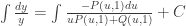 where
where  (here, P and Q are from the general form
  ). Well, it turns out that if you plug the coefficients from my example into those equations, the denominator will become 0 for each one. So I (obviously) need to check for that
  and
and  are not 0 before running the homogeneous coefficients solver on a differential equation.
 or
or  in them, and they are now automatically reduced to just
  . Of course, the disadvantage to this, as I mentioned in the other post, is that it will only simplify once. Also, I wrote the function very specifically for expressions returned by dsolve. It only works, for example, with constants named sequentially like C1, C2, C3 and so on. Even with making it specialized, it was still hell to write. I was also able to get it to renumber the constants, so something like
  with
with  and find the roots of it. Then you plug the roots into an exponential times
  for i from 1 to the multiplicity of the root (as in
  ). You usually expand the real and complex parts of the root using Euler’s Formula, and, once you simplify the constants, you get something like
  for each i from 1 to the multiplicity of the root. Anyway, with the new constantsimp() routine, I was able to set this whole thing up as one step, because if the imaginary part is 0, then the two constants will be simplified into each other. Also, SymPy has some good polynomial solving, so I didn’t have any problems there. I even made good use of the collect() function to factor out common terms, so you get something like
  instead of
  , which for larger order solutions, can make the solution much easier to read (compare for example,
  with the expanded form,
  as the solution to
  ).
).  . The method will set up an integral to represent the particular solution to any equation of this form, assuming that you have all
  cannot be zero (otherwise it would be a n-1 order ODE), so we can and should divide through by it. Lets pretend that we already did that, and just use the same letters. Also, I will rewrite
  to emphasize that the coefficients do not have to be constants for this to work. So you have your linear inhomogeneous ODE:
  . So, as I mentioned above, we need n linearly independent solutions to the homogeneous equation
  to use this method. Let us call those solutions
  . Now let us write our particular solution as
  . Now, if we substitute our particular solution in to the left hand side of our ODE, we should get
 as a summation to help keep things from getting too messy. I am also going to write
  instead of
  on terms for additional sanity. Every variable is a function of x.
  . The particular solution should satisfy the condition of the ODE, so
 .
.
 .
. .
. terms in individually of the
  . Now the
  terms will vanish because we can factor out a
  for each j from 0 to n-2, then this will take care of this; the terms with higher derivatives on


 .
. . So this is where it is nice that I learned
  , or
, or  , where
  is the Wronskian of the fundamental system with the ith column replaced with
  . So we finally have
  .
.  . So implementing it was easy enough. But it soon became clear that there would be some problems with this method. Sometimes, the SymPy would return a really simple Wronskian, something like
  , but other times, it would return something crazy. For example, consider the expression that I reported in
 ") .
. , which is the set of linearly independent solutions to the ODE
  . Well, the problem here is that, as verified by Maple, that complex Wronskian above is identically equal to
  . SymPy’s
  (see the issue page for more information on this). Unfortunately, SymPy’s
  , which is the second derivative of
  with respect to x. According to the example file, it is know as Einstein’s equations. Maple has a nice
  term, which is perfectly reasonable as that term will never be 0. You can then make the substitution
  , and you will reduce the order of the ODE to first order, which in this case would be a Bernoulli equation, the first thing that I ever implemented in SymPy.
  , then the solution to the ODE is
 for some function or x and y
  generates equations of that type, so it could be actually useful for solving other things.
  is the term under the square root of the famous solution
  . It is clear that a quadratic has repeated roots if and only if the discriminant is 0. Well, the same is true for the discriminant of any polynomial. I am not highly familiar with this (ask me again after I have taken my abstract algebra class next semester), but apparently there is something called the resultant, which is the product of the differences of roots between two polynomials and which can also be calculated without explicitly finding the roots of the polynomials. Clearly, this will be 0 if and only if the two polynomials share a root. So the discriminant is built from the fact that a polynomial has a repeated root iff it shares a root with its resultant. So it is basically the resultant of a polynomial and its derativave, times an extra factor. It is 0 if and only if the polynomial has a repeated root.
